$ \newcommand\vu{\mathbf{u}} \newcommand\vv{\mathbf{v}} \newcommand\vw{\mathbf{w}} \newcommand\vi{\mathbf{i}} \newcommand\vj{\mathbf{j}} \newcommand\vk{\mathbf{k}} \newcommand\vo{\mathbf{o}} \newcommand\vr{\mathbf{r}} \newcommand\vt{\mathbf{t}} \newcommand\vx{\mathbf{x}} \newcommand\vy{\mathbf{y}} \newcommand\vz{\mathbf{z}} \newcommand\va{\mathbf{a}} \newcommand\vb{\mathbf{b}} \newcommand\vc{\mathbf{c}} \newcommand\ve{\mathbf{e}} \newcommand{\vE}{\mathbf{E}} \newcommand{\vS}{\mathbf{S}} \newcommand{\vk}{\mathbf{k}} \newcommand{\vq}{\mathbf{q}} \newcommand{\vzero}{\mathbf{0}} \newcommand{\vomega}{\mathbf{ω}} \newcommand{\mI}{\mathbf{I}} \newcommand{\mM}{\mathbf{M}} \newcommand{\mR}{\mathbf{R}} \newcommand{\mP}{\mathbf{P}} \newcommand{\mK}{\mathbf{K}} \newcommand{\mW}{\mathbf{W}} \DeclareMathOperator{\Tr}{Tr} \newcommand{\abs}[1]{\left\lvert {#1} \right\rvert} \newcommand{\norm}[1]{\left\lVert {#1} \right\rVert} \newcommand{\ensemble}[1]{\left\langle {#1} \right\rangle} \newcommand{\der}[2]{\frac{\partial {#1}}{\partial {#2}}} \newcommand{\Der}[2]{\frac{\delta {#1}}{\delta {#2}}} \newcommand{\lap}{\nabla^2} $

Lecture notes in polymer physics

This material is based on the lectures given by Prof. A. C. Shi from Jan. 12 to 14, 2009 at Fudan University, with some additional derivation details.


Download Fulltext in PDF

1. One Mode Approximation


Assume the function to be approximated can be expanded in a series

\[\phi (x) = \sum_n \phi_n (x) e^{ik_nx}\]

where \(n = 0, \pm 1, \pm 2, \cdots\). For one mode approximation, only the first three terms are taken, that is

\[\phi (x) = \phi_0 (x) e^{ik_0x} + \phi_{-1} (x) e^{ik_{-1}x} + \phi_1 (x) e^{ik_1x}\]

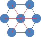
In two and higher dimensional space, variables, \(x\) and \(k\), become vectors \(\mathbf{x}\) and \(\mathbf{k}\). To approximate high dimensional functions, one should consider the origin and its neighbors. Using two-dimensional hexagonal lattice as an example, one mode approximation retains only the origin term and the six nearest neighbors, depicted in Figure 1.

matplotlib default output
Figure 1

One mode approximation is not a good approximation for square wave. To expand square wave function according to eq. 1, \(\phi_n\) decrease with \(n\) in an order of \(1/n\), which is very slow and a large number of terms are required to approximate it well enough. This also explains that spectral method is not suitable to deal with strong segregation systems where the density profile resembles a square wave function.

2. Spinodal Decomposition and Nucleation


3. Conserved and Non-conserved Order Parameter


4. Ginzburg Criteria


5. Scattering Theory


6. Excluded Volume and Incompressibility


7. Structure Factor for Single Ideal Gaussian Chain


8. Response Function and Fluctuation-Dissipation Theorem


9. Random Phase Approximation


10. Landau Theory and Phase Transition


11. Variational Mean-Field Theory


12. Perturbation Theory


13. Weak Segregation Theory and Strong Segregation Theory


14. Saddle Point Approximation