Rotations and their representations

Julia in Practice: Building Scattering.jl from Scratch (4)

Yi-Xin Liu 2020-04-18 Research · Software · Tutorials Julia Scattering.jl Scattering Theory

In this post we implement submodules rotation.jl of Scattering.jl to rotate a vector in the reference coordinate system to the internal coordinate system of the scatterer. Three representations of a rotaion operation are discussed and implemented. The conversion among and math operations on these representations are also implemented.

Rotations
Implementation
Usage
Acknowledgements
References

Rotations

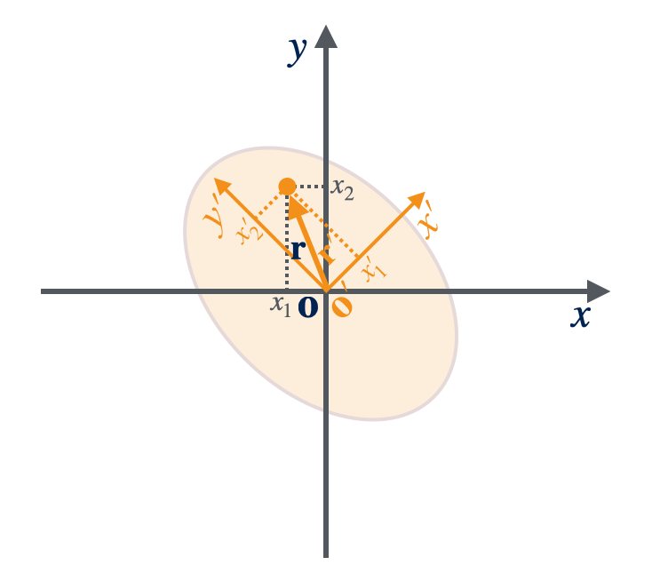
Rotations are another type of isometric transformation which preserve distances and angles. As stated in the previous post, we will adopt the convention of alias transformation. Therefore, a rotation operation is applied to the coordinates. It will rotate the reference coordinates to the internal coordinates of a scatterer. It thus natural to choose a rotation to represent the orientation of a scatterer, as shown in Figure 1. In the following, we will briefly review three popular represenations of a rotation. For a more comprehensive introduction, especially in the context of crystallography, please consult these references¹². A series of Wiki pages about rotations in a general sense are also good sources to learn:

Figure 1. Illustration for rotation of the reference coordinate system to the internal coordinate system of a scatterer.

Rotation matrices

The transformation of a position vector $\vr = [x\;y\;z]^T = [x_1\;x_2\;x_3]^T$ in the reference coordinate system $xyz$ to the internal coordinate system of a scatterer $x’y’z’$ can be written as a multiplication of the vector by a rotation matrix $\mR$. The resulted position vector $\vr’=[x’\;y’\;z’]^T$ with its coordinates expressed in the $x’y’z’$ system is then given by

\[\vr' = \mR\vr\]

To determine the rotation matrix which has 9 components in 3D space, we have to identify at least 9 equations. It is most convenient to examine the transformation of three basis vectors of the $x’y’z’$ system, $\vu=[u_x\;u_y\;u_z]^T, \vv=[v_x\;v_y\;v_z]^T, \vw=[w_x\;w_y\;w_z]^T$ with their coordinates expressed in the $xyz$ system. When the coordinates of these basis vectors are expressed in the $x’y’z’$ system, they are just three unit vectors $[1\;0\;0]^T, [0\;1\;0]^T, [0\;0\;1]^T$. Thus we have

\[\begin{equation} \begin{split} \mR\vu &= [1\;0\;0]^T \\ \mR\vv &= [0\;1\;0]^T \\ \mR\vw &= [0\;0\;1]^T \end{split} \end{equation}\]

It is possible to rewrite above equation in a more compact form as

\[\begin{equation} \begin{split} \mR[\vu\;\vv\;\vw] &= \begin{bmatrix} 1& 0& 0 \\ 0& 1& 0 \\ 0& 0& 1 \end{bmatrix} \\ &= \mI \end{split} \end{equation}\]

The term in the right hand side of the above equation is just an identity matrix $\mI$. In convention, we will write the matrix $[\vu\;\vv\;\vw]$ as $\mP$. Obviously, $\mP$ is an orthonormal matrix because its three column vectors are just three basis vectors of a coordinate system which are unit vectors and orthogonal to each other. As long as we know all the components of the three basis vectors of the internal coordinate system in the reference coordinate system, we can easily construct $mP$ and the rotation matrix can be obtained by inverse the above equation:

\[\mR = \mP^{-1}\]

This equation can be futher simplified using a property of an orthornormal matrix:

\[\begin{equation} \begin{split} \mP^T\mP &= \begin{bmatrix} \vu^T \\ \vv^T \\ \vw^T \end{bmatrix} [\vu\;\vv\;\vw] \\ &= \mI \end{split} \end{equation}\]

which means

\[\mP^{-1} = \mP^T\]

Therefore, the rotation matrix is just the transposition of $\mP$:

\[\begin{equation} \mR = \mP^T = \begin{bmatrix} u_x& u_y& u_z \\ v_x& v_y& v_z \\ w_x& w_y& w_z \end{bmatrix} \end{equation}\]

It is now clear that $\mP$ is also a rotation matrix which transforms a vector in the internal coordinate system to the reference coordinate system. All rotation matrices should have following properties:

$\mR^{-1} = \mR^T$
$\det(\mR) = \pm 1$ since $1=\det(I)=\det(\mR^T\mR)=\det(\mR^T)\det(\mR)=\det(\mR)^2$

For the coordinate system transformation described above, the determinat should be the volume of the parallelopiped which is $+1$. such $\mR$ is called a proper rotation. Given a matrix, to determine whether it is a proper rotation matrix, we should first compute its determinant to see if it is $+1$. If so, we then compute its inverse, and check if it is identical to its transposition. If both crierions are met, then the matrix represents a proper rotation in the Cartesian coordinate system. However, it is not necessary true for other non-Cartesian coordinate systems.

Euler axis angle

The rotation matrix is convenient for numerical computations, however it is not an intuitive way to represent a rotation. The most popular way to describe a rotation is by Euler axis angle or polar angles: there exists a rotation axis given by a unit vector $\vomega$, about which the object rotates by angle $\theta$ according to the Euler’s rotation theorem.

Rotation axis

By definition, a vector $\vr$ parallel to the rotation axis is invariant under rotation:

\[\mR\vr = \vr\]

\[\begin{equation} (\mR - \mI)\vr = 0 \end{equation}\label{eq:rotaxis0}\]

Obviously, the vector $\vr$ is an eigenvector of $\mR$ corresponding to the eigenvalue $\lambda=+1$. To obtain $\vr$, we can simply diagonalize $\mR$ and find the eigenvector corresponding to the eigenvalue of $+1$. For non-symmetric $\mR$, however, there is a simpler way to determine $\vr$. We can show that

\[\begin{equation} \begin{split} (\mR - \mR^T)\vr &= [(\mI - \mR^T) + (\mR - \mI)]\vr \\ &= (\mI - \mR^T)\vr + (\mR - \mI)\vr \\ &= (\mR^T\mR - \mR^T)\vr + (\mR - \mI)\vr \\ &= \mR^T(\mR - \mI)\vr + (\mR - \mI)\vr \\ &= \mR^T 0 + 0 \\ &= 0 \end{split} \end{equation}\label{eq:skewsym}\]

From the second to the third line, we have invoked the property of a rotation matrix $\mR^T\mR = \mI$, while from the fourth to the fifth line eq.\eqref{eq:rotaxis0} is applied. It is also easy to show that $\mR - \mR^T$ is a skew-symmetric matrix because

\[(\mR - \mR^T)^T = \mR^T - \mR = -(\mR - \mR^T)\]

A skew-symmetric matrix can be used to represent cross products as matrix multiplications. Consider vectors $\va = [a_1\;a_2\;a_3]^T$ and $\vb = [b_1\;b_2\;b_3]^T$. Then, defining a skew-symmetric matrix with its components from $\va$

\[\begin{equation} [\va]_{\times} = \begin{bmatrix} 0& -a_3& a_2 \\ a_3& 0& -a_1 \\ -a_2& a_1& 0 \end{bmatrix} \end{equation}\label{eq:crossproduct}\]

the cross product can be written as

\[\va \times \vb = [\va]_{\times}\vb.\]

Since the cross product of any vector with itself is equal to 0, eq.\eqref{eq:skewsym} implies that $\mR - \mR^T$ is actually the cross product matrix of vector $\vr$,

\[\mR - \mR^T = [\vr]_{\times}.\]

By writing out $\mR - \mR^T$ explicitly as

\[\begin{equation} \mR - \mR^T = \begin{bmatrix} 0& u_y-v_x& u_z-w_x \\ v_x-u_y& 0& v_z-w_y \\ w_x-u_z& w_y-v_z& 0 \end{bmatrix} \end{equation}\label{eq:RRT}\]

Comparing eq.\eqref{eq:RRT} with eq.\eqref{eq:crossproduct}, we immediately arrives at

\[\begin{equation} \vr = \begin{bmatrix} r_x \\ r_y \\ r_z \end{bmatrix} = \begin{bmatrix} w_y-v_z \\ u_z-w_x \\ v_x-u_y \end{bmatrix} = \begin{bmatrix} R_{32}-R_{23} \\ R_{13}-R_{31} \\ R_{21}-R_{12} \end{bmatrix} \end{equation}\label{eq:vomega}\]

The last term is useful when we denote the rotation matrix as $\mR = [R_{ij}]$ where $i={1,2,3},j={1,2,3}$ are row and column indices, respectively. Finally, the unit vector parallel to the rotation axis is

\[\begin{equation} \vomega = \frac{\vr}{\norm{\vr}} \end{equation}\label{eq:vomega-norm}\]

Note that $\vomega$ computed by eq.\eqref{eq:vomega} becomes a zero vector when $\mR$ is symmetric. Therefore, this approach is inapplicable to symmetric matrices.

Rotation angle

Once the rotation axis is known, the angle of rotation $\theta$ is the angle between two vectors $\va$ and $\mR\va$, where $\va$ can be any vector that is perpendicular to $\vomega$.

However, a more straightforward way to find $\theta$ is to compute the trace of the rotation matrix and invoke the relation²

\[\begin{equation} \Tr(\mR) = 1 + 2\cos\theta \end{equation}\label{eq:trR}\]

It follows that the angle of rotation can be computed via

\[\begin{equation} \theta = \arccos\left[ \frac{\Tr(\mR)-1}{2} \right] \end{equation}\label{eq:theta}\]

where we should restrict the range of $\theta$ to $[0, \pi]$.

Conversion to the rotation matrix

Given by an Euler axis angle representation with known $\vomega=[\omega_x\;\omega_y\;\omega_z]^T$ and $\theta$, we can construct the corresponding rotation matrix directly:

\[\begin{equation} \mR = \begin{bmatrix} \cos\theta + \omega_x^2(1-\cos\theta)& \omega_x\omega_y(1-\cos\theta)-\omega_z\sin\theta& \omega_x\omega_z(1-\cos\theta)+\omega_y\sin\theta \\ \omega_y\omega_x(1-\cos\theta)+\omega_z\sin\theta& \cos\theta + \omega_y^2(1-\cos\theta)& \omega_y\omega_z(1-\cos\theta)-\omega_x\sin\theta \\ \omega_z\omega_x(1-\cos\theta)-\omega_y\sin\theta& \omega_z\omega_y(1-\cos\theta)+\omega_x\sin\theta& \cos\theta + \omega_z^2(1-\cos\theta) \end{bmatrix} \end{equation}\label{eq:aa2rm}\]

See ref² for how to derive above equation. Alternatively, we can utilize the cross product matrix of $\vomega$ by comparing to eq.\eqref{eq:crossproduct}:

\[\begin{equation} \mK = \begin{bmatrix} 0& -\omega_z& \omega_y \\ \omega_z& 0& -\omega_x \\ -\omega_y& \omega_x& 0 \end{bmatrix} \end{equation}\label{eq:Kmat}\]

The rotation matrix is then obtained as

\[\begin{equation} \mR = \mI + \mK\sin\theta + (1-\cos\theta)\mK^2 \end{equation}\label{eq:K2rm}\]

The above equation can be derived in a Lie-algebraic way or a geometric way using the Rodrigues’ rotation formula.

Euler angles

Another popular description of a rotation is using Euler angles. It is demonstrated by Leonhard Euler that it is sufficient to rotate a reference coordinate system by three angles around three axes of a coordinate system to reach any target frame. The rotation around an axis of a coordinate system is called an elemental/basic rotation. Albeit its popularity, the Euler angles representation of a rotation causes many confusions and it has a serious artifact known as the Gimbal lock. There exist twelve possible sequences of rotation axes, leading to twelve conventions. Different fields usually choose a particular convention. In this project, we will choose the Z1Y2Z3 convention according to the Wiki page Euler angles.

Convert Euler angles to the rotation matrix

Euler angles are denoted as $\alpha, \beta, \gamma$. The rotation matrix conforming to the Z1Y2Z3 convention has the form

\[\begin{equation} \mR = \begin{bmatrix} \cos\alpha\cos\beta\cos\gamma-\sin\alpha\sin\gamma& -\cos\gamma\sin\alpha-\cos\alpha\cos\beta\sin\gamma& \cos\alpha\sin\beta \\ \cos\alpha\sin\gamma+\cos\beta\cos\gamma\sin\alpha& \cos\alpha\cos\gamma-\cos\beta\sin\alpha\sin\gamma& \sin\alpha\sin\beta \\ -\cos\gamma\sin\beta& \sin\beta\sin\gamma& \cos\beta \end{bmatrix} \end{equation}\label{eq:euler2mat}\]

Convert the rotation matrix to Euler angles

From eq.\eqref{eq:euler2mat}, we have

\[\begin{split} \frac{R_{23}}{R_{13}} &= \tan\alpha \\ R_{33} &= \cos\beta \\ \frac{R_{32}}{-R_{31}} &= \tan\gamma \end{split}\]

Then Euler angles can be obtained acoordingly

\[\begin{equation} \begin{split} \alpha &= \arctan(R_{23}, R_{13}) \\ \beta &= \arccos(R_{33}) \\ \gamma &= \arctan(R_{32}, -R_{31}) \end{split} \end{equation}\label{eq:mat2euler}\]

where $\arctan(a, b)$ is a specialized version of the arctan function which takes into account the quadrant that the point $(b, a)$ is in. Note that eq.\eqref{eq:mat2euler} is valid for $\theta$ in the range $(0, \pi]$. When $\beta=0$ or $R_{33}=1$, $\alpha$ and $\gamma$ has infinite many solutions which satisfy

\[\tan(\alpha+\gamma) = \frac{R_{21}}{R_{11}}\]

\[\alpha + \gamma = \arctan(R_{21}, R_{11})\]

In this project, we fix $\gamma=0$ when $\beta=0$.

Implementation

It is now straightforward to implement a submodule rotation.jl of Scattering.jl which realize rotations and their associated operations.

Rotation types

First, we define an abstract type to describe any rotation operators:

1
abstract type AbstractRotation end

Inheriting from it, we define a concrete type for rotation matrices:

1
2
3
struct RotationMatrix{T<:Real} <: AbstractRotation
    R::RotMatrix{T} # 3x3 matrix
end

To ensure the user supplied matrix is actually a rotation matrix, we add an internal constructor to it

1
2
3
4
5
6
7
function RotationMatrix(R::RotMatrix{T}) where {T<:Real}
    # Verify that P is a valid rotation matrix
    detR = det(R)
    @assert(detR ≈ one(detR), "Not a valid rotation matrix: det=$detR.")
    @assert(transpose(R) ≈ inv(R), "Not a valid rotation matrix: RT != R^-1.")
    new{T}(R)
end

It is convenient to define a outer constructer which takes three arguments. They are unit basis vectors of the internal coordinate system of a scatterer $\vu, \vv, \vw$ whose components are expressed in the reference coordinate system.

1
RotationMatrix(u::Vector3D{T}, v::Vector3D{T}, w::Vector3D{T}) where {T <: Real} = RotationMatrix(transpose(RotMatrix(hcat(u,v,w))))

Note that we first construct $\mP$ using hcat function. Then we transpose it to obtain $\mR$ using transpose function.

Similarly, we define a concrete type for Euler axis angle:

1
2
3
4
5
struct EulerAxisAngle{T<:Real} <: AbstractRotation
    ω::RVector{T} # rotation axis
    θ::T # in radian unit
    K::SMatrix{3,3,T} # the cross product matrix such that Kv = ω×v for any vector v.
end

Note that the cross product matrix $\mK$ is also stored. We also need an internal constructor which ensures the rotation axis vector is a unit vector

1
2
3
4
5
function EulerAxisAngle(ω::RVector{T}, θ::T) where {T<:Real}
    ω /= norm(ω) # make sure ω is normalized
    K = hcat([0, ω[3], -ω[2]], [-ω[3], 0, ω[1]], [ω[2], -ω[1], 0])
    new{T}(ω, θ, K)
end

Finally, we define a concrete type for Euler angles:

1
2
3
4
5
struct EulerAngle{T<:Real} <: AbstractRotation
    α::T # in radian unit
    β::T # in radian unit
    γ::T # in radian unit
end

And an internal constructor is also necessary to ensure all three angles are in the same type:

1
2
3
function EulerAngle(α::T=0, β::T=0, γ::T=0) where {T<:Real}
    new{T}(α, β, γ)
end

Conversions

Conversions are implemented as outer constructors for each type. Converting Euler axis angle to a rotation matrix:

1
2
3
4
5
6
function RotationMatrix(axisangle::EulerAxisAngle)
    θ = axisangle.θ
    K = axisangle.K
    R = one(K) + sin(θ)*K + (1-cos(θ))*K*K
    RotationMatrix(R)
end

where eq.\eqref{eq:K2rm} is used. Converting Euler angles to a rotation matrix:

1
2
3
4
5
6
7
8
9
10
11
12
13
function RotationMatrix(euler::EulerAngle)
    c1 = cos(euler.α)
    c2 = cos(euler.β)
    c3 = cos(euler.γ)
    s1 = sin(euler.α)
    s2 = sin(euler.β)
    s3 = sin(euler.γ)
    v1 = [c1*c2*c3 - s1*s3 -c3*s1 - c1*c2*s3 c1*s2]
    v2 = [c1*s3 + c2*c3*s1 c1*c3 - c2*s1*s3 s1*s2]
    v3 = [-c3*s2 s2*s3 c2]
    R = RotMatrix(vcat(v1, v2, v3))
    RotationMatrix(R)
end

where eq.\eqref{eq:euler2mat} is used. Converting a rotation matrix to Euler axis angle:

1
2
3
4
5
6
7
8
9
10
11
12
13
14
function EulerAxisAngle(rotmatrix::RotationMatrix)
    R = rotmatrix.R
    θ = acos((tr(R)-1)/2)
    v = [R[3,2]-R[2,3], R[1,3]-R[3,1], R[2,1]-R[1,2]]
    if θ ≈ zero(θ)
        return EulerAxisAngle([1.0, 0.0, 0.0], 0.0)
    end
    if v ≈ zero(v)
        vals, vecs = eigen(R)
        idx = findfirst(x -> x ≈ one(x), vals)
        ω = real(vecs[:, idx])
    end
    EulerAxisAngle(ω, θ)
end

where eq.\eqref{eq:vomega} and eq.\eqref{eq:theta} are used. Converting a rotation matrix to Euler angles:

1
2
3
4
5
6
7
8
9
10
11
12
13
function EulerAngle(rotmatrix::RotationMatrix)
    R = rotmatrix.R
    if R[3,3] ≈ one(R[3,3])
        α = atan(R[2,1],R[1,1])
        β = zero(α)
        γ = zero(α)
    else
        α = atan(R[2,3], R[1,3])
        β = acos(R[3,3])
        γ = atan(R[3,2], -R[3,1])
    end
    EulerAngle(α, β, γ)
end

where eq.\eqref{eq:mat2euler} is used.

The conversions between Euler angles and Euler axis angle are implemented by converting them to rotation matrices first:

1
2
EulerAxisAngle(euler::EulerAngle) = RotationMatrix(euler) |> EulerAxisAngle
EulerAngle(axisangle::EulerAxisAngle) = RotationMatrix(axisangle) |> EulerAngle

Strictly follow our convention developed in this post, the conversions among these three representations are lostless. Thus it is reasonable to define a set of conversion rules following the Julia guidelines:

1
2
convert(::Type{T}, x::AbstractRotation) where {T<:AbstractRotation} = T(x)
convert(::Type{T}, x::T) where {T<:AbstractRotation} = x

The second line handles the situation when the object x is already of the target type.

Promotion

The rotation matrix is most convenient for numerical compuations. Therefore, its rank is considered higher than the other two representations. It means that we will convert any type of a rotation to the rotation matrix during computation. In Julia, it is realized by promotion rules. A promotion rule promote two or more types to a single common type. It will be used implicitly by Julia for methods promote_type and promote.

We define the following promotion rule:

1
promote_rule(::Type{T}, ::Type{S}) where {T<:AbstractRotation, S<:AbstractRotation} = RotationMatrix

which promotes two rotations of different types to the RotationMatrix type. However, when two rotations are of same type, Julia implicitly does nothing and this behavior can not be overridden at present. For example, if two rotations are of type EulerAngle, the return type will be EulerAngle instead of RotationMatrix. It is important to bare this in mind when implement == and * later.

It is also convenient to implement a promote method which takes a single argument and promotes all rotations to the RotationMatrix type. Note that one-argument promote is not supported by Julia Base.

1
2
promote(rot::RotationMatrix) = rot
promote(rot::AbstractRotation) = RotationMatrix(rot)

Inversion

The inversion of a rotation is computed via inverting the rotation matrix, then converting it back to the original type:

1
2
inv(rot::RotationMatrix) = collect(transpose(rot.R)) |> RotationMatrix
inv(rot::T) where {T<:AbstractRotation} = inv(promote(rot)) |> T.name.wrapper

In the above implementation, we utilized the relation $\mR^{-1} = \mR^T$.

Comparison

It is meaningful to check whether two rotations are identical. So we have extended the == operator defined in Julia Base:

1
2
3
4
==(rot1::RotationMatrix, rot2::RotationMatrix) = rot1.R ≈ rot2.R
==(rot1::EulerAngle, rot2::EulerAngle) = RotationMatrix(rot1) == RotationMatrix(rot2)
==(rot1::EulerAxisAngle, rot2::EulerAxisAngle) = RotationMatrix(rot1) == RotationMatrix(rot2)
==(rot1::AbstractRotation, rot2::AbstractRotation) = ==(promote(rot1,rot2)...)

Note how poromtion rules defined previously has been used.

Multiplication of two rotation operations

Since any rotation operation can be expressed as a matrix, it means that we can multiply them together to obtain another rotation. Mulitiplication of two rotations of any type is implemented by first promoting them to the RotationMatrix type:

1
2
3
4
*(rot1::RotationMatrix, rot2::RotationMatrix) = RotationMatrix(rot1.R * rot2.R)
*(rot1::EulerAngle, rot2::EulerAngle) = RotationMatrix(rot1) * RotationMatrix(rot2)
*(rot1::EulerAxisAngle, rot2::EulerAxisAngle) = RotationMatrix(rot1) * RotationMatrix(rot2)
*(rot1::AbstractRotation, rot2::AbstractRotation) = *(promote(rot1,rot2)...)

Note that the result of a multiplication is always of type RotationMatrix. As mentioned earlier, promotion of two rotations of an identical type returns this type other than RotationMatrix. Therefore, it is required to explicitly add the first three lines.

Power of a rotation operation

Raising a rotation to an integral power $n$ means multiplying a rotation for $n$ times. A naive implementation is

1
2
3
4
5
6
7
8
function pow1(rot::AbstractRotation, n::Integer)
    rot = promote(rot)
    result = rot
    for i in 1:(n-1)
        result *= rot
    end
    result
end

However, the complexity is only $O(N)$. The complexity can be optimized to $O(\log(N))$:

1
2
3
4
5
6
7
8
9
10
11
12
13
14
15
function ^(rot::AbstractRotation, n::Integer)
    rot = promote(rot)
    if n == zero(n)
        return one(rot)
    elseif n == one(n)
        return rot
    else
        if isodd(n)
            return rot * rot^(n-1)
        else
            rothalf = rot^(n÷2)
            return rothalf * rothalf
        end
    end
end

where we have utilized a unit rotation which is simply a do-nothing rotation. It is implemented as follows:

1
2
one(rot::RotationMatrix{T}) where {T<:Real} = one(rot.R) |> RotationMatrix
one(rot::T) where {T<:AbstractRotation} = one(promote(rot)) |> T.name.wrapper

Using BechmarkTools, we can compare these two methods as

julia> using BenchmarkTools
julia> using Scattering
julia> # construct euler ...
julia> @btime pow1($euler, 1000)
142.561 μs (3004 allocations: 172.31 KiB)
julia> @btime $euler^1000
2.327 μs (49 allocations: 3.02 KiB)

We can see that the optimized version is nearly $70\times$ faster than the naive version when $n=1000$.

Transformation of a position vector

Transformation of a position vector with components expressed in the reference coordinate system to the internal coordinate system of a scatterer is implemented by applying a rotation operation on the vector:

1
*(rot::AbstractRotation, v::RVector{T}) where {T <: Real} = promote(rot).R * v

As can be seen, the actual computation is carried out by a matrix-vector product.

Usage

Due to the length of this blog post, the usage as well as the test of rotation.jl is presented in a separate blog post.

Acknowledgements

This work is partially supported by the General Program of the National Natural Science Foundation of China (No. 21873021).

References

Wondratschek, H. Matrices, Mappings and Crystallographic Symmetry. In IUCr Commission on Crystallographic Teaching: Teaching pamphlets; 1997. ↩
Evans, P. R. Rotations and Rotation Matrices. Acta Cryst. D 2001, 57, 1355–1359. ↩ ↩² ↩³

Table of Contents