Fundamentals of X-Ray Scattering
Julia in Practice: Building Scattering.jl from Scratch (5)
In this post we will present a concise review of the fundamental theory of X-ray scattering, including electromagnetic waves, flux and intensity, scattering cross section and scattering length, scattering by an electron, interference, and atomic form factor. Although the specific properties of X-rays are used, the derivation is applicable to other incident beams, such as neutrons. The derivation presented here is different from most of literature with an emphasis on a consistent treatment on the wave nature of the incident beam. The notations used in this post mostly follow the book by Roe1.
Table of Contents
Electromagnetic Wave
An electromagnetic wave, including X-rays, which is monochromatic, sinusoidal, and planar travelling, has the following form:
\[\begin{equation} \vE(\vr,t) = \vE_0\cos(\omega t - \vk\cdot\vr) \end{equation}\label{eq:waveE}\]where $\vE_0$ is a constant vectors, $\vk$ is called the wave vector, and $\omega$ is the angular frequency. The frequency in hertz, $\nu$, is related to the angular frequency via
\[\omega = 2\pi\nu\]Actually, it is more convenient to write
\[\begin{equation} \vE(\vr,t) = \vE_0 e^{i(\omega t - \vk\cdot\vr)} \end{equation}\label{eq:wave}\]where, by convention, the electromagnetic wave is the real part of the above equation.
The direction of the wave vector $\vk$ is the direction of the wave travels and its length is $2\pi/\lambda$. Thus the wave vector is sometimes written as
\[\begin{equation} \vk = \frac{2\pi}{\lambda}\vS \end{equation}\label{eq:vk}\]where $\vS$ is a unit vector and $\lambda$ is the wave length which is related to the frequency as
\[\lambda = \frac{c}{\nu}\]Here $c$ is the speed of light.
The amplitude of an electromagnetic wave is
\[\begin{equation} E(\vr, t) = E_0 \cos(\omega t - \vk\cdot\vr) \end{equation}\label{eq:ampE}\]where $E_0=\abs{\vE_0}$. It is also more convenient to write it in a complex form
\[\begin{equation} A(\vr, t) = E_0 e^{i(\omega t - \vk\cdot\vr)} \end{equation}\label{eq:ampA}\]where it is understood that the actual amplitude is the real part of $A$: $E(\vr,t)=\mathrm{Real}[A(\vr,t)]$. Note that, however, the amplitude is not equal to $\abs{A}$ which is just $E_0$.
Flux
Flux of a plane wave
The energy density of an electromagnetic plane wave is given by
\[u(\vr, t) = \epsilon_0\abs{\vE}^2.\]where $\epsilon_0$ is the permittivity in vacuum. This energy density moves with the electric and magnetic fields in a similar manner to the wave itself. We can find the rate of transport of energy, i.e., the flux, by considering a small time interval $\Delta t$. A wave passes through a cylinder of length $c\Delta t$ and cross-sectional area $S$ in the interval $\Delta t$. The energy passing through area $S$ in time $\Delta t$ is
\[u \times (\mathrm{volume\;of\;the\;cylinder}) = uSc\Delta t\]The energy per unit area per unit time passing through an area perpendicular to the wave, called the energy flux and denoted by $j$, can be calculated by dividing the energy by the area $S$ and the time interval $\Delta t$:
\[j = \frac{uSc\Delta t}{S\Delta t} = cu\]or
\[\begin{equation} j = c\epsilon_0\abs{\vE}^2 \end{equation}\]By substituting eq.\eqref{eq:ampE} into above equation, we have
\[j(\vr, t) = c\epsilon_0 E_0^2 \cos^2(\omega t - \vk\cdot\vr)\]$j$ is an extremely rapidly varying quantity since the frequency is of the order of $10^{19}$ Hz with the fact that the typical wave length of an X-ray radiated by a copper target tube is 0.154 angstrom. In X-ray scattering experiments, we are most interested in the time averaged flux $J$. Since the wave is a periodic function of time with a period of $T=2\pi/\omega$, the time arerage can be simply carried out in a full cycle starting at $\vr=0$:
\[\begin{equation} \begin{split} J &= \ensemble{j} \\ &= \frac{1}{T}\int_0^Tdt\;j(t) \\ &= c\epsilon_0 E_0^2 \frac{1}{T}\int_0^Tdt\; \cos^2(\frac{2\pi} {T}t) \\ &= \frac{1}{2}c\epsilon_0 E_0^2 \end{split} \end{equation}\label{eq:JE02}\]It can be seen that the time averaged flux is proportional to the square of the maximum amplitude of the electromagnetic wave. Therefore, by utilizing eq.\eqref{eq:ampA}, we can rewrite above equation into
\[J = \frac{1}{2}c\epsilon_0 AA^*\]where $A^*$ is the complex conjugate of $A$. However, it is more common to absorb the constants $c\epsilon_0/2$ into $A$. Thus, later on throughout this project, we will define the amplitude of an electromagnetic wave as
\[\begin{equation} A(\vr, t) = A_0 e^{i(\omega t - \vk\cdot\vr)} \end{equation}\label{eq:finalA}\]where
\[\begin{equation} A_0 = \left( \frac{1}{2}c\epsilon_0 \right)^{1/2} E_0 \end{equation}\label{eq:A0}\]And the (time averaged) flux can now be simply written as
\[\begin{equation} J = \abs{A}^2 = AA^* \end{equation}\label{eq:JAA}\]Flux of a spherical wave
In a typical experimental setup for X-ray scattering as shown in Figure 1, the incident beam is always a plane wave. Such plane wave irradiates a sample, from which the scattered beam emanates in all directions.
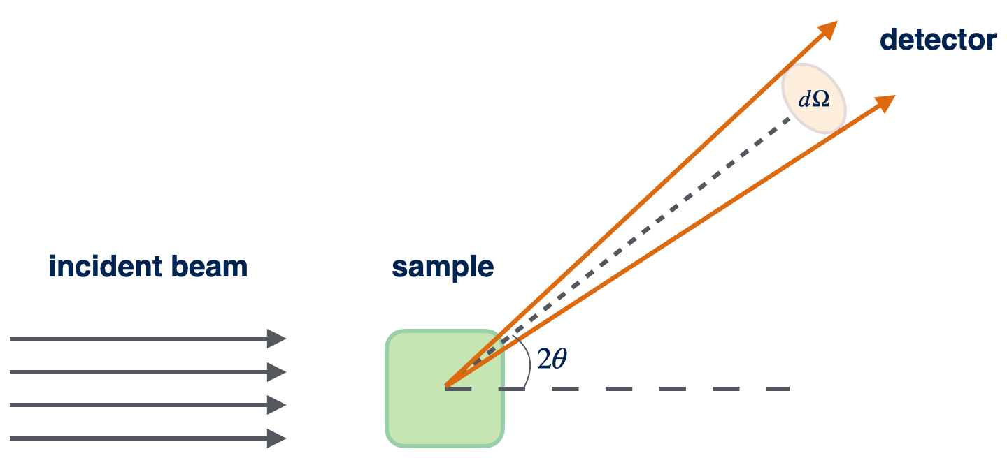
Experimentally we measure the flux of the scattered beam as a function of the scattering angle denoted as $2\theta$. The scattered beam is a spherical wave. Before we discuss the flux of a spherical wave. Let’s first get familiar with the concept of the solid angle.
Just like a planar angle in radians is the ratio of the length of a circular arc to its radius, the solid angle is defined as
\[\begin{equation} \Omega = \frac{S}{R^2} \end{equation}\label{eq:Omega}\]Here, $S$ is the spherical surface area and $R$ is the radius of the considered sphere. In particular, for a full spherical surface, its solid angle is $\Omega=4\pi R^2 / R^2 = 4\pi$. The solid angle for a cone with its apex at the apex of the solid angle, and with apex angle $2\theta$ is given by
\[\Omega = 2\pi(1-\cos\theta).\]The flux of a spherical wave is invariant only when it passing through a solid angle. It can be easily seen by considering the beam as a steam of photons. Obviously, the number of photons emanating from a point source is a constant passing through a solid angle. Thus the flux in the unit of solid angle is
\[\begin{equation} J_{\Omega} = \frac{nE_p}{\Omega} \end{equation}\label{eq:JOmega}\]while the flux in the unit of area is
\[J = \frac{nE_p}{S}\]where $E_p$ is the energy of a photon. Inserting it into eq.\eqref{eq:JOmega} and using eq.\eqref{eq:Omega}, we then have
\[\begin{equation} J_{\Omega} = JR^2 \end{equation}\label{eq:JOmegaJ}\]Note that, for a spherical wave, the relation between flux and the maximum magnitude of a plane wave in eq.\eqref{eq:JAA} should be rewritten as
\[\begin{equation} J_\Omega = \abs{A}^2 = AA^*. \end{equation}\label{eq:JOmegaAA}\]Scattering by an electron
Suppose a free electron is placed at position O, as shown in Figure 2. The incident X-ray beam propagates in the direction of the $x$ axis. Its flux is $J_0$ in the unit of per area since it is a plane wave. The incident beam is scattered by the electron and the scattering wave is observed at position P by a detector. As compared to the wavelength of the X-ray, the distance $R = OP$ is large. The scattering angle $2\theta$ is the angle between line OP and the $x$ axis. In all following derivations, the scattering event is considered to be both coherent and no phase change occurs.
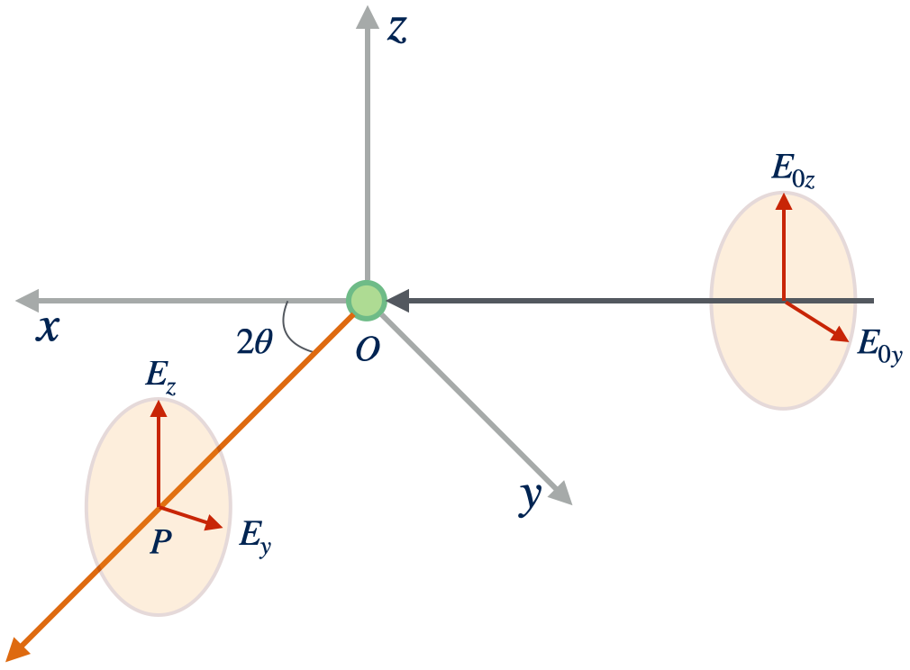
The full wave representation of the incident beam is given by eq.\eqref{eq:wave}. The electric field vector $\vE_0$ should be in the $yz$ plane perpendicular to the propagating direction of the incident beam because the electromagnetic wave is a transverse wave. To identify the scattering wave at angle $2\theta$, the task is to determine its maximum amplitude and its phase.
Maximum magnitude of the scattered wave
The vector $\vE_0$ in arbitrary direction can be decomposed into two vectors parallel to the $y$ and $z$ axes, respectively. Let’s first consider the case in which the incident beam is polarized in the $z$ direction, with the maximum magnitude being $E_{0z}$. The electromagnetic field of the beam sets the free electron oscillating in the $z$ direction. The alternating acceleration of the oscillating electron in turn induces emission of an electromagnetic wave of the same frequency propagating in all directions. According to the classic electromagnetic theory, the maximum magnitude of the scattering wave at position P obeys
\[\begin{equation} E_z = E_{0z}\frac{e^2}{mc^2}\frac{1}{R} \end{equation}\label{eq:Ez}\]where $e$ and $m$ are the charge and mass of an electron, respectively.
Next, Let’s consider a incident beam with its electric field vector pointing to the $y$ direction. In this case, the oscillation of the electron is no longer perpendicular to the line OP. Thus the electric field vector $\vE_y$ is the projection of the vector $\vE_{0y}$ on to the line perpendicular to both $z$ axis and the line OP. From Figure 2, it is easily seen that the angle between the vector $\vE_{0y}$ and $\vE_y$ is $2\theta$, thus the magnitude of $\vE_y$ is
\[\begin{equation} E_y = E_{0y}\frac{e^2}{mc^2}\frac{1}{R}\cos2\theta. \end{equation}\label{eq:Ey}\]For an arbitrarily polarized incident beam, it can be expressed as
\[\begin{equation} \vE_0 = \vE_{0y} + \vE_{0z}. \end{equation}\label{eq:E0}\]The $y$ and $z$ components of $\vE_0$ contributes in the scattering wave in the way given by eq.\eqref{eq:Ez} and eq.\eqref{eq:Ey}. Then the electric field vector of the scattering wave is $\vE = \vE_y + \vE_z$, and its magnitude is
\[\begin{equation} E^2 = E_y^2 + E_z^2 = \frac{e^2}{mc^2}\frac{1}{R}\left( E_{0z}^2 + E_{0y}^2\cos^22\theta \right) \end{equation}\]For an unpolarized beam, the direction of its electric field varies randomly with time. We are most interested in the time average value of the scattering wave:
\[\begin{equation} \ensemble{E^2} = \ensemble{E_y^2} + \ensemble{E_z^2} = \left(\frac{e^2}{mc^2}\right)^2 \frac{1}{R^2}\left( \ensemble{E_{0z}^2} + \ensemble{E_{0y}^2}\cos^22\theta \right) \end{equation}\label{eq:E2}\]To find $\ensemble{E_{0y}^2}$ and $\ensemble{E_{0z}^2}$, we invoke the following relation using eq.\eqref{eq:E0}:
\[E_0^2 = E_{0y}^2 + E_{0z}^2\]and taking time average of both sides of the above equation
\[E_0^2 = \ensemble{E_0^2} = \ensemble{E_{0z}^2} + \ensemble{E_{0y}^2}\]However, since the beam is randomly polarized, the time average of $y$ and $z$ components should be equal. Thus we have
\[\ensemble{E_{0z}^2} = \ensemble{E_{0y}^2} = \frac{1}{2}E_0^2\]Inserting above equation into eq.\eqref{eq:E2}, we arrive at
\[\begin{equation} \ensemble{E^2} = E_0^2\left(\frac{e^2}{mc^2}\right)^2\frac{1+\cos^22\theta}{R^2} \end{equation}\label{eq:E2_avg}\]Scattering cross section and scattering length
According to eq.\eqref{eq:JE02}, with $\ensemble{E^2}$ given by eq.\eqref{eq:E2_avg}, the flux in the unit of per area is
\[J = \frac{1}{2}c\epsilon_0\ensemble{E^2}=\frac{1}{2}c\epsilon_0E_0^2\left(\frac{e^2}{mc^2}\right)^2\frac{1+\cos^22\theta}{2R^2}\]Using eq.\eqref{eq:JOmegaJ}, the flux in the unit of per solid angle is then
\[\begin{equation} J_\Omega = JR^2 = \frac{1}{2}c\epsilon_0E_0^2\left(\frac{e^2}{mc^2}\right)^2\frac{1+\cos^22\theta}{2} \end{equation}\label{eq:JOmega_electron}\]This is called the Thomson formula for the scattering of X-rays by a single free electron. The flux of the incident plane wave is given by eq.\eqref{eq:JE02} and we repeat it here
\[J_0 = \frac{1}{2}c\epsilon_0E_0^2\]We now define a quantity, the differential scattering cross section of an electron for unpolarized x-rays, as
\[\begin{equation} \left(\frac{d\sigma}{d\Omega}\right)_e = \frac{J_\Omega}{J_0} = \left(\frac{e^2}{mc^2}\right)^2\frac{1+\cos^22\theta}{2} \end{equation}\label{eq:crosssection}\]Since $J_\Omega$ has the unit of reciprocal of solid angle and $J$ has the unit of reciprocal of area, the differential scattering cross section has a unit of area. Taking the square root of it, the result is in unit of length which is called the scattering length
\[\begin{equation} b_e = \frac{J_\Omega}{J_0} = \frac{e^2}{mc^2} \left(\frac{1+\cos^22\theta}{2}\right)^{1/2} \end{equation}\label{eq:be}\]In fact, the above derivation is applicable to any charged particles, such as nucleus. However, as the scattering length $b_e$ is proportional to $1/m^2$, the scattering by nucleus is negligible because the mass of a nucleon is much higher than the electron. Thus the scattering of x-rays from matter results entirely from the presence of electrons around atomic centers.
By comparing eq.\eqref{eq:JOmega_electron} to eq.\eqref{eq:JOmegaAA}, we find the maximum magnitude of a scattering wave is given by
\[\begin{equation} A_0b_e \end{equation}\label{eq:magnitude}\]where $A_0$ is defined in eq.\eqref{eq:A0}.
Phase of the scattering wave
Figure 3 shows the paths travelled by the incident beam and the scattering wave at scattering angle $2\theta$. The phase difference between the wave at position Q and at the position of the beam source P is given by
\[\Delta\phi_1 = \vk_0\cdot(\vr - \vr_0),\]while the phase difference between the wave at the detector D and at position Q is given by
\[\Delta\phi_2 = \vk\cdot(\vr_d - \vr).\]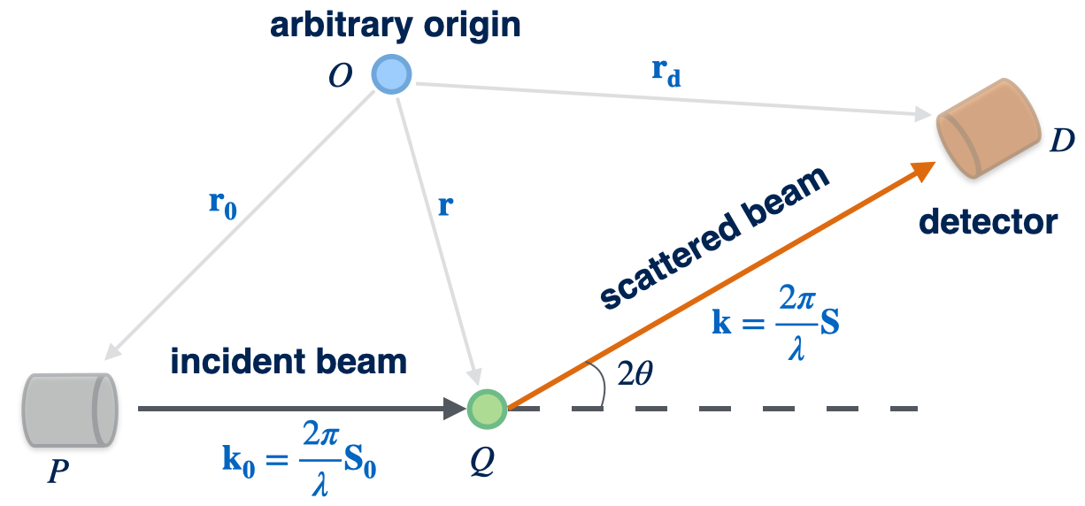
The total phase difference between the scattering wave reaching the detector and the incident wave leaving the beam source is
\[\begin{equation} \begin{split} \Delta\phi &= \Delta\phi_1 + \Delta\phi_2 \\ &= \vk_0\cdot(\vr - \vr_0) + \vk\cdot(\vr_d - \vr) \\ &= (\vk\cdot\vr_d-\vk_0\cdot\vr_0) - (\vk - \vk_0)\cdot\vr \\ &= f(2\theta) - (\vk - \vk_0)\cdot\vr \end{split} \end{equation}\label{eq:Deltaphi}\]The last line of the above equation tells us that the total phase difference consists of two parts: the first part is independent of the position of the electron (scatterer) and the second part is a function of $\vr$. It is common to define a scattering vector
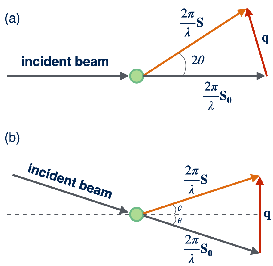
\[\begin{equation} \vq = \vk - \vk_0 = \frac{2\pi}{\lambda}(\vS - \vS_0) \end{equation}\]Its relation with the incident beam and the scattering wave is illustrated in Figure 4. Figure 4b shows that the scattering vector is perpendicular to the angular bisector of the angle of the other two wave vectors.
We then write the incident beam at the beam source
\[\vE_{P}(t) = \vE_0e^{i(\omega t - \vk_0\cdot\vr_0)}\]Its phase is
\[\begin{equation} \phi_P = \omega t - \vk_0\cdot\vr_0 \end{equation}\label{eq:phiP}\]Consequently, we can compute the phase of the scattering wave reaching the detector, using eq.\eqref{eq:Deltaphi}, as
\[\begin{equation} \begin{split} \phi_D &= \phi_P + \Delta\phi \\ &= (\omega t - \vk_0\cdot\vr_0) + (\vk\cdot\vr_d-\vk_0\cdot\vr_0) - \vq\cdot\vr \\ &= \omega t + g(2\theta) - \vq\cdot\vr \end{split} \end{equation}\label{eq:phiD}\]With the maximum magnitude given by eq.\eqref{eq:magnitude} and the phase given by the above equation, the amplitude of the scattering wave reaching the detector is
\[\begin{equation} A = A_0b_e e^{i[\omega t + g(2\theta) - \vq\cdot\vr]} \end{equation}\label{eq:amplitude}\]Interference
When a beam of x-rays irradiates a sample, it usually results in two different phenomena: (1) scattering of x-rays by a single electron which is described in the previous section, and (2) interference among the waves scattered by these primary events. This interference essentially leads to the variation of the fluxes of the waves scattered in different directions. In experiments, we measure the flux as a function of the scattering direction and the relative placement of electrons or atoms in the sample are readily deduced from the collected data.
Strictly speaking, the term scattering should refer only to phenomenon (1) above, whereas the term diffraction refers to the combination of phenomena (1) and (2). However, this distinction is seldom followed and these two terms are often used interchangeably. In practice, the term diffraction is used only for crystalline samples or when the structure of the sample is sufficiently regular to exhibit sharp peaks in the scattering curve. When the scattering pattern is diffuse, and especially when the pattern of interest is mainly in the small-angle region, the term scattering is almost exclusively used although the phenomenon (2) inevitably presented.
In this section, we shall develop a formalism for treatment of phenomenon (2). A derivation different from most of literature is presented first. The classical derivation is also discussed for the sake of completeness.
Derivation based on formula \eqref{eq:amplitude}
Once we have the formula eq.\eqref{eq:amplitude} for an electron at any position $\vr$, we can compute the total amplitude of all scattering waves at scattering angle $2\theta$, scattered by $N$ electrons positioned at $\vr_n$ for $n=1,2,\dots,N$, reaching the detector simply by adding all amplitudes together:
\[A = \sum_{n=1}^N A_n = \sum_{n=1}^N A_0b_e e^{i[\omega t + g(2\theta) - \vq\cdot\vr_n]}\]We can moving all terms that are independent of $n$ outside of the summation, leading to
\[A = A_0b_e e^{i[\omega t + g(2\theta)]}\sum_{n=1}^N e^{-i\vq\cdot\vr_n}\]It follows that the flux of the scattering wave at angle $2\theta$ is
\[\begin{split} J_\Omega &= AA^* \\ &= \left[ A_0b_e e^{i[\omega t + g(2\theta)]}\sum_{n=1}^N e^{-i\vq\cdot\vr_n]} \right]\left[ A_0b_e e^{i[\omega t + g(2\theta)]}\sum_{n=1}^N e^{-i\vq\cdot\vr_n]} \right]^* \\ &= A_0^2b_e^2 \sum_{n=1}^N e^{-i\vq\cdot\vr_n} \sum_{n=1}^N e^{i\vq\cdot\vr_n} \end{split}\]From the second line to the third line, the factors $e^{i[\omega t + g(2\theta)]}$ and $e^{-i[\omega t + g(2\theta)]}$ cancels out. Since these factors make no contribution to the flux, without losing any information, we can write the amplitude in a simpler form
\[\begin{equation} A(\vq) = A_0b_e\sum_{n=1}^N e^{-i\vq\cdot\vr_n} \end{equation}\label{eq:ANelectrons}\]where $\vr_i$ is the position vector of the $i$-th electron. When the number of electrons is large and they distributed more or less continuously in the space, we can convert the above equation into an integral by defining a number density operator (field) of electrons:
\[n_e(\vr) = \sum_{n=1}^N \delta(\vr-\vr_n)\]where $\delta(x)$ is a delta function. To see that $n_e(\vr)$ is actually a number density, we integrate it and find that the result is the number of electrons $N$ as expected:
\[\begin{split} \int d\vr\; n_e(\vr) &= \int d\vr\; \sum_{n=1}^N \delta(\vr-\vr_n) \\ &= \sum_{n=1}^N \int d\vr\;\delta(\vr-\vr_n) \\ &= \sum_{n=1}^N 1 \\ &= N \end{split}\]where from the second line to the third line, we have used the definition of a delta function $\int dx\;\delta(x)=1$. The particular property of the delta function we will use here is
\[f(x_0) = \int dx\; f(x)\delta(x-x_0)\]Using above equation, we can rewrite $e^{-i\vq\cdot\vr}$ as
\[e^{-i\vq\cdot\vr_n} = \int d\vr\; e^{-i\vq\cdot\vr} \delta(\vr-\vr_n)\]Inserting this equation into eq.\eqref{eq:ANelectrons}, we have
\[\begin{split} A &= A_0b_e\sum_{n=1}^N \int d\vr\; e^{-i\vq\cdot\vr} \delta(\vr-\vr_n) \\ &= A_0b_e \int d\vr\; e^{-i\vq\cdot\vr} \sum_{n=1}^N \delta(\vr-\vr_n) \\ &= A_0b_e \int d\vr\; n_e(\vr) e^{-i\vq\cdot\vr} \end{split}\]or
\[\begin{equation} A(\vq) = A_0b_e \int_V d\vr\; n_e(\vr) e^{-i\vq\cdot\vr} \end{equation}\label{eq:Aintegral}\]where $V$ denotes that the integration to be performed over the scattering volume. This equation shows that the wave amplitude $A(\vq)$ is proportional to the 3D Fourier transform of the number density $n_e(\vr)$ of the electrons. The Fourier transform plays a central role in the interpretation of scattering and diffraction phenomena.
Classical derivation
The classical derivation of the total amplitude of the scattering waves at angle $2\theta$ reaching the detector considers the setup shown in Figure 5, where two electrons are placed at two positions O and P. The scattering waves emitted by electron $O$ and electron $P$ are both in the direction of the wave vector $\vk$. The angle between the wave vector of the incident beam $\vk_0$ and $\vk$ is $2\theta$.
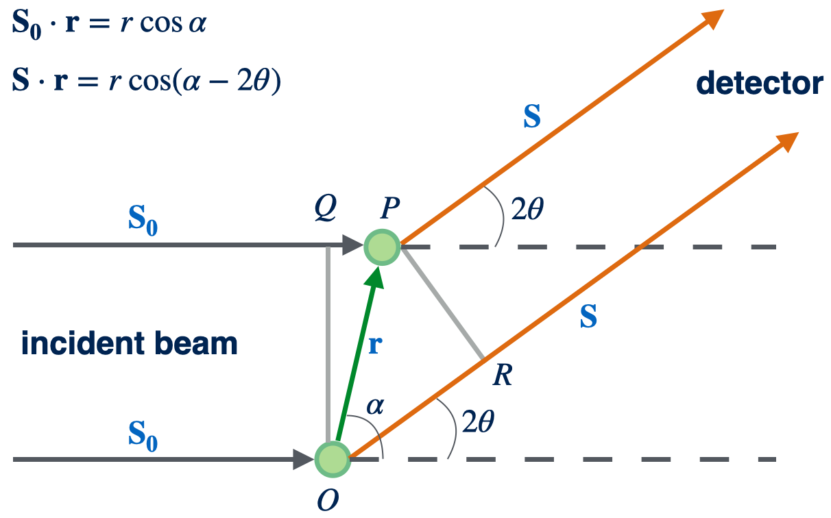
From the discussion presented in the previous section, we know that the maximum magnitudes of both scattering waves arriving at the detector are identical. But their phase difference $\Delta\phi$ will depend on the path length difference $\delta$ between the two waves:
\[\Delta\phi = \phi_P - \phi_O = \frac{2\pi}{\lambda}\delta\]From Figure 5, we find the path length difference is
\[\delta = QP - OR\]Note that in the above equation we write the length $QP$ first because in the definition of $\Delta\phi$ we put P at first. To compute the length $QP$, we designate a vector pointing from O to P as $\vr$ which is the difference of the position vectors of position O and P: $\vr = \vr_P - \vr_O$. Then we have $QP = \vS_0\cdot\vr$ and $OR=\vS\cdot\vr$. Therefore, the phase difference can be expressed in terms of $\vS, \vS_0$ and $\vr$ as
\[\begin{split} \Delta\phi &= \frac{2\pi}{\lambda}(\vS_0\cdot\vr - \vS\cdot\vr) \\ &= -(\frac{2\pi}{\lambda}\vS - \frac{2\pi}{\lambda}\vS_0)\cdot\vr \\ &= -\vq\cdot\vr \end{split}\]where the scattering vector $\vq$ is naturally obtained. Assume that the amplitude of the spherical wave $A_O(x,t)$ scattered at point O is
\[\begin{equation} A_O(x,t) = A_0b_e e^{i(\omega t - 2\pi x/\lambda)} \end{equation}\label{eq:AO}\]where $x$ is understood as the path travelled along the direction $\vS$. Because of the phase difference, the amplitude of the spherical wave $A_P(x,t)$ scattered at point P is then
\[\begin{split} A_P(x,t) &= A_O(x,t)e^{i\Delta\phi} \\ &= A_0b_e e^{i(\omega t - 2\pi x/\lambda)}e^{i\Delta\phi} \end{split}\]The combined wave $A(x,t)$ that reaches the detector is the sum of $A_O(x,t)$ and $A_P(x,t)$:
\[\begin{split} A(x,t) &= A_O(x,t) + A_P(x,t) \\ &= A_0b_e e^{i(\omega t - 2\pi x/\lambda)}(1 + e^{-i\vq\cdot\vr}) \end{split}\]Then the flux is evaluated as
\[\begin{split} J_\Omega(\vq) &= A(x,t)A_P^*(x,t) \\ &= A_0^2b_e^2 (1 + e^{i\vq\cdot\vr})(1 + e^{-i\vq\cdot\vr}) \end{split}\]where the phase factors $e^{i(\omega t - 2\pi x/\lambda)}$ and $e^{-i(\omega t - 2\pi x/\lambda)}$ cancels out. It is thus suffice to write the amplitude of the scattering wave as
\[\begin{equation} A(\vq) = A_0b_e(1 + e^{-i\vq\cdot\vr}) \end{equation}\label{eq:Aclassical}\]When there are $N$ electrons, eq.\eqref{eq:Aclassical} can easily be generalized to
\[A(\vq) = A_0b_e \sum_{n=1}^N e^{-i\vq\cdot\vr_n}\]which is exactly the same as eq.\eqref{eq:ANelectrons}. In the above equation, $\vr_n$ denotes the position of electron $n$ relative to an arbitrary origin. When eq.\eqref{eq:Aclassical} was derived, the origin was placed at one of the electrons, but that was not necessary. What really matters is only the relative difference in the path length between the rays scattered at different electrons. Any effect of the change in the origin would have simply canceled out when the flux was evaluated by taking the absolute square of the amplitude.
It can be seen that the classical derivation is not as clear as our single electron scattering based derivation. For example, the amplitude expressions presented in eq.\eqref{eq:AO} and related are implicitly assumed without any proof. By comparing to eq.\eqref{eq:amplitude}, we know that $x$ in eq.\eqref{eq:AO} has a much deeper meaning than it seems.
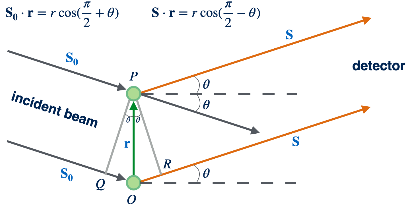
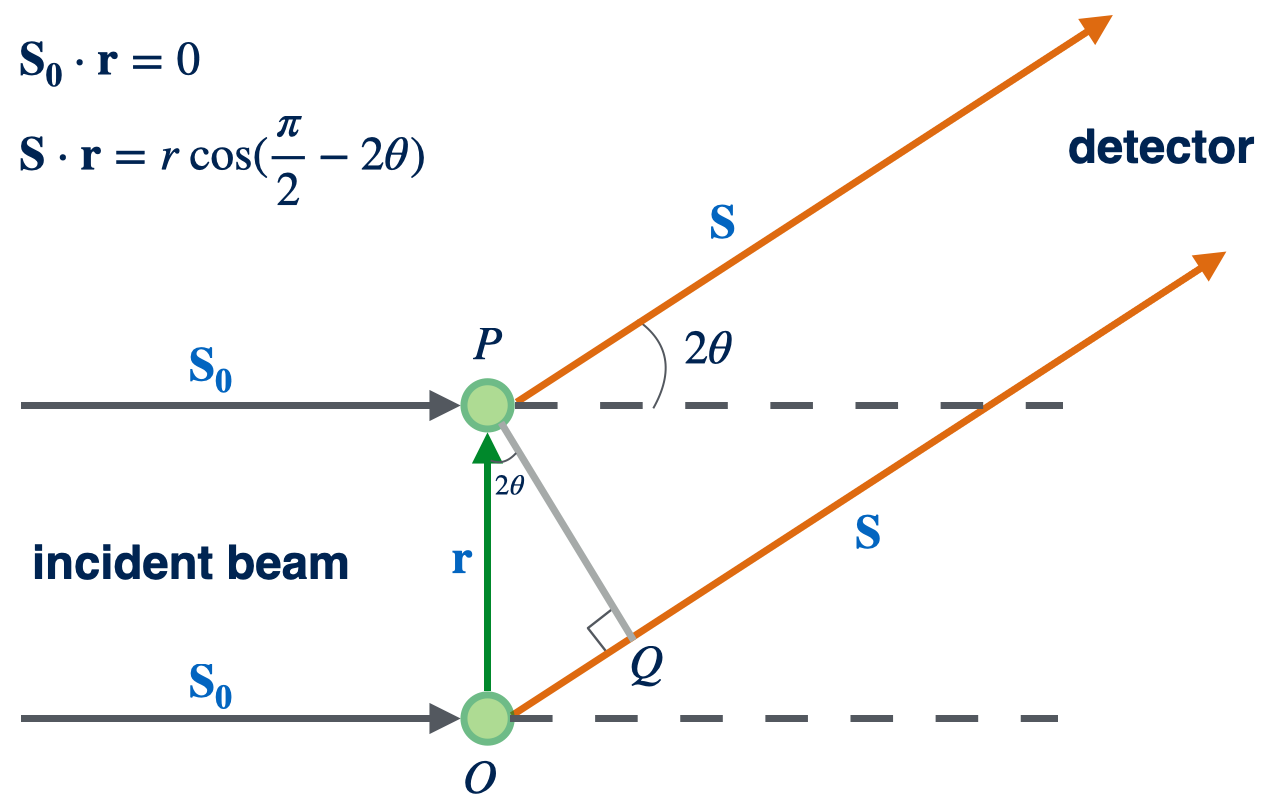
In the previous derivation, it is assumed that the incident beam and the vector $\vr$ forms an arbitrary angle $\alpha$, shown in Figure 5. In the derivation of the Bragg’s law in the crystallographic community, a specific $\alpha=\pi/2 + \theta$ is assumed as shown in Figure 6, which simplifies the calculation of the path difference. It should be bared in mind, however, that such setup is not general. Another popular setup to develop the scattering theory is shown in Figure 7, where $\alpha$ is chosen to be $\pi/2$ which is another special case of the setup shown in Figure 5.
Scattering by Atoms
The amplitude of x-ray scattering from an atom can be directly obtained by viewing the atom as a cluster of electrons and using eq.\eqref{eq:ANelectrons} or eq.\eqref{eq:Aintegral}. Note that the x-ray scattering from the atomic nucleus can be ignored as discussed in the previous section.
Atomic form factor
The atomic form factor is defined as the amplitude of x-ray scattering from an atom measured in the unit of $A_0b_e$:
\[\begin{equation} f(\vq) = \frac{A(\vq)}{A_0b_e} = \int d\vr\; n_e(\vr) e^{-i\vq\cdot\vr} \end{equation}\label{eq:atom}\]where $n_e(\vr)$ is the time-averaged electron density distribution of the atom, and $\vr$ is defined by putting the origin of the reference coordinate system on the center of the atom. For a free atom, $n_e(\vr)$ bares spherical symmetry. Consequently, the atomic form factor only depends on the magnitude of the scattering vector. By expressing eq.\eqref{eq:atom} in a spherical coordinate system and performing integration over inclination and azimuth, we find
\[\begin{split} f(q) &= \int_0^{2\pi}d\phi\int_0^{\pi}d\theta\;\sin\theta \int_0^{\infty}dr\; n_e(r)r^2 e^{-iqr\cos\theta} \\ &= 2\pi\int_0^{\infty}dr\; n_e(r)r^2 \int_0^{\pi}d\theta\;\sin\theta e^{-iqr\cos\theta} \\ &= 2\pi\int_0^{\infty}dr\; n_e(r)r^2 \int_0^{\pi}d(-\cos\theta)\; e^{-iqr\cos\theta} \\ &= 2\pi\int_0^{\infty}dr\; n_e(r)r^2 \left[ \frac{e^{-iqr\cos\theta}}{iqr} \right]_0^{\pi} \\ &= 2\pi\int_0^{\infty}dr\; n_e(r)r^2\frac{e^{iqr}-e^{-iqr}}{iqr} \\ &= 2\pi\int_0^{\infty}dr\; n_e(r)r^2\frac{2i\sin(qr)}{iqr} \\ &= 4\pi\int_0^{\infty}dr\; n_e(r)r^2\frac{\sin(qr)}{qr} \end{split}\]or
\[\begin{equation} f(q) = 4\pi\int_0^{\infty}dr\; n_e(r)r^2\frac{\sin(qr)}{qr} \end{equation}\]where we have chosen the polar axis of the spherical coordinate system to coincide with the direction of $\vq$, and the origin at the atom center.
Multiple atoms
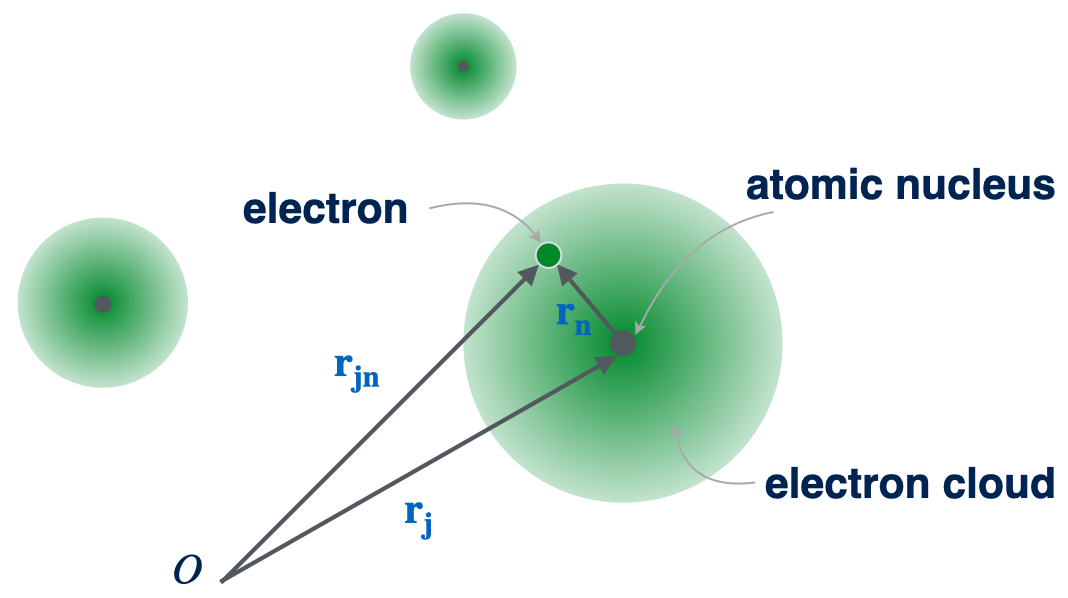
For x-ray scattering by multiple atoms, it is convenient to regroup electrons according to atoms to which they belong to. As shown in Figure 8, the position vector $\vr_{jn}$ of any electron can be decomposed into two parts:
\[\vr_{jn} = \vr_j + \vr_n\]where $\vr_j$ is the position vector of the center of $j$th atom ($j=1, 2, \dots, N_a$), and $\vr_n$ denotes the relative position of $jn$th electron ($n=1, 2, \dots, Z_j$) with respect to the center of $j$th atom.
With this setup, eq.\eqref{eq:ANelectrons} can be rewritten as
\[\begin{split} A(\vq) &= A_0b_e \sum_{j=1}^{N_a} \sum_{n=1}^{Z_j} e^{-i\vq\cdot\vr_{jn}} \\ &= A_0b_e \sum_{j=1}^{N_a} \sum_{n=1}^{Z_j} e^{-i\vq\cdot(\vr_j+\vr_n)} \\ &= A_0b_e \sum_{j=1}^{N_a} \left(\sum_{n=1}^{Z_j} e^{-i\vq\cdot\vr_n}\right) e^{-i\vq\cdot\vr_j} \end{split}\]The quantity in the parentheses in the third line of above equation, when averaged over time, is in effect the same as the integral presented in eq.\eqref{eq:atom}. Therefore, we can write the above equation as
\[\begin{equation} A(\vq) = A_0b_e \sum_{j=1}^{N_a} f_j(\vq) e^{-i\vq\cdot\vr_j} \end{equation}\label{eq:atoms}\]where $f_j(\vq)$ denotes the atomic form factor of $j$th atom. If the sample has only one type of atom, we can factor out the $f_j$ term because $f(\vq)=f_j(\vq)$ is independent of $j$:
\[\begin{equation} A(\vq) = A_0b_ef(\vq) \sum_{j=1}^{N_a} e^{-i\vq\cdot\vr_j} \end{equation}\label{eq:sameatoms}\]Similar to the number density operator for electrons, we introduce a number density operator defined for the center of atoms:
\[n_a(\vr) = \sum_{j} \delta(\vr-\vr_j)\]which enable us to write eq.\eqref{eq:sameatoms} in the form
\[\begin{equation} A(\vq) = A_0b_e f(\vq) \int_Vd\vr\; n_a(\vr) e^{-i\vq\cdot\vr} \end{equation}\label{eq:sameatomsintegral}\]Now it is reasonable to define a scattering length of an atom:
\[\begin{equation} b_a = b_e f(\vq) \end{equation}\label{eq:ba}\]which transforms eq.\eqref{eq:sameatomsintegral} to
\[\begin{equation} A(\vq) = A_0b_a \int_Vd\vr\; n_a(\vr) e^{-i\vq\cdot\vr} \end{equation}\label{eq:generalsameatoms}\]Eq.\eqref{eq:generalsameatoms} has an exactly same form as eq.\eqref{eq:Aintegral} by the mapping $b_a \to b_e$ and $n_a(\vr) \to n_e(\vr)$. Note that $b_a$ is in general a function of $\vq$.
Furthermore, we can define a scattering length density distribution of an atom as
\[\begin{equation} \rho_a(\vr) = b_a n_a(\vr) \end{equation}\label{eq:rhoa}\]which further reduce eq.\eqref{eq:generalsameatoms} to
\[\begin{equation} A(\vq) = A_0 \int_Vd\vr\; \rho_a(\vr) e^{-i\vq\cdot\vr} \end{equation}\label{eq:finalsameatoms}\]If there are $M$ types of atoms, each has $N_{a\alpha}$ atoms with $\alpha=1, 2, \dots, M$. Each atom of type $\alpha$ has $Z_\alpha$ electrons. Thus the total number of electrons in the sample is
\[N = Z_\alpha \sum_{\alpha=1}^{M} N_{a\alpha}\]Eq.\eqref{eq:atoms} is linear with respect to the index of atom $j$, which means that the amplitude of each type of atom can be simply added to obtain the total amplitude. Therefore, the most general form of the amplitude of x-ray scattering from a collection of atoms is
\[\begin{equation} A(\vq) = A_0b_e \sum_{\alpha=1}^{M} f_\alpha(\vq) \int_Vd\vr\; n_{a\alpha}(\vr) e^{-i\vq\cdot\vr} \end{equation}\label{eq:generalatoms}\]where $n_{a\alpha}(\vr)$ is the number density distribution of the atom of type $\alpha$. With the definition of scattering length density distribution of the atom $\rho_{a\alpha}$ for the atom of type $\alpha$, we can write eq.\eqref{eq:generalatoms} in a more compact form:
\[\begin{equation} A(\vq) = A_0 \int_Vd\vr\; \rho(\vr) e^{-i\vq\cdot\vr} \end{equation}\label{eq:finalatoms}\]with the scattering length distribution of the sample $\rho(\vr)$ defined by
\[\begin{split} \rho(\vr) &= \sum_{\alpha=1}^{M} \rho_{a\alpha}(\vr) \\ &= \sum_{\alpha=1}^{M} b_{a\alpha} n_{a\alpha}(\vr) \\ &= \sum_{\alpha=1}^{M} b_e f_\alpha(\vq) n_{a\alpha}(\vr) \end{split}\]Clearly the scattering length distribution of the sample $\rho(\vr)$ is a sum of the products of the scattering length of an electron $b_e$, the atomic form factor $f_\alpha(\vq)$, and the number density of the atom $n_{a\alpha}(\vr)$, for each type of atom.
Generalization to Arbitrary Particles
The strategy described in the Multiple atoms section can be generalized to arbitrary particles consisting of any type of building blocks, such as electrons, atoms, molecules, complexes, polymers, nanoparticles, etc., as long as they can be viewed as basic building blocks of the sample. Such generalization will eventually lead to the concept of form factor, which we will pursue further in the next post.
Acknowledgements
This work is partially supported by the General Program of the National Natural Science Foundation of China (No. 21873021).
References
-
Roe, R. J. Methods of X-Ray and Neutron Scattering in Polymer Science; Oxford University Press, 2000. ↩